Vector Search: HNSW, IVF and Approximate Nearest Neighbours
On this page
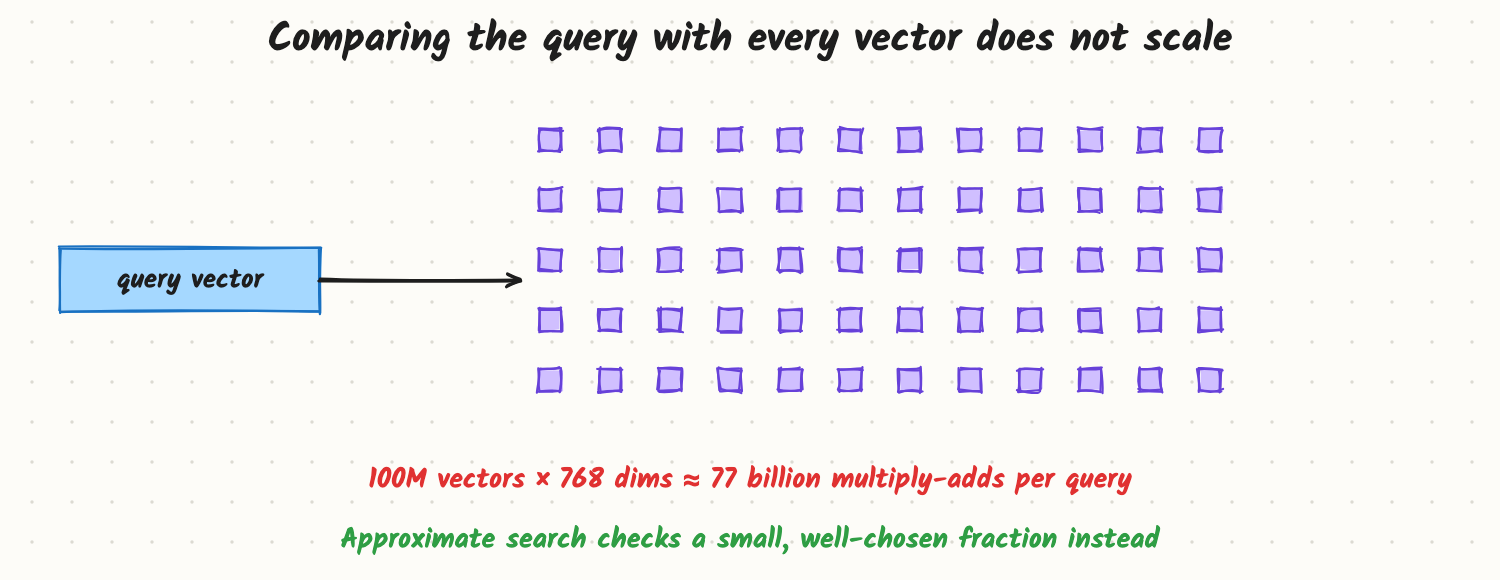
Semantic search works beautifully on 10,000 documents: embed the query, compare it with every stored vector, return the closest. At 100 million chunks the same approach means roughly 77 billion multiply-adds per query, hundreds of milliseconds or more even on fast hardware, and the raw vectors don't fit in one machine's memory. Approximate nearest neighbour (ANN) indexes trade a tiny bit of accuracy for searches that are orders of magnitude faster.
How it works
The trade: recall for speed
Exact (brute-force) search always finds the true nearest neighbours. ANN indexes find most of them while looking at a small fraction of the data. Quality is measured as recall@k: of the true top k, how many did the index return? Production systems usually tune for something like 0.9–0.99 recall at a latency budget.
IVF: cluster, then search nearby clusters
An inverted file index (IVF) first groups the vectors into clusters (with k-means) and remembers each cluster's centre (centroid). At query time:
- Compare the query with the centroids only (a few thousand, not millions).
- Pick the
nprobeclosest clusters. - Search the vectors in those clusters exhaustively.
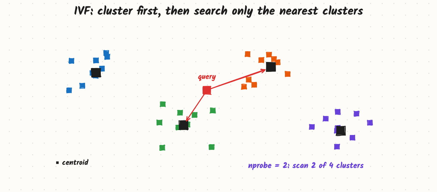
IVF is simple, fast to build and works well with compression. Its weak spot: a true neighbour sitting just across a cluster boundary is missed unless nprobe is high enough.
HNSW: a layered graph you walk greedily
Hierarchical Navigable Small World (HNSW) connects each vector to a handful of near neighbours, forming a graph, and adds sparser layers on top with long-range links (like express lanes).
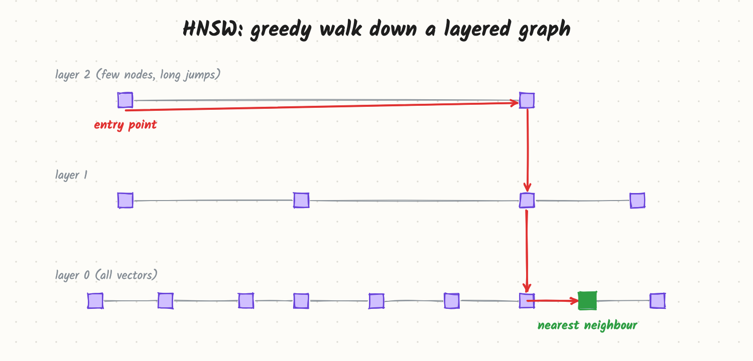
A query starts at an entry point on the top layer, repeatedly moves to whichever neighbour is closer to the query, drops a layer when no neighbour is closer, and ends with a small candidate list at layer 0. Key settings:
- M: links per node (more links, better recall, more memory);
- efConstruction: effort when building;
- efSearch: size of the candidate list at query time (the main recall/latency knob).
HNSW gives excellent recall at low latency and supports inserts easily, but it keeps full vectors plus the graph in memory, and deletes are awkward.
Compression: product quantization
Product quantization (PQ) splits each vector into sub-vectors and replaces each with the ID of its nearest "code" from a small learned codebook, shrinking a 3 KB float vector to tens of bytes. Distances are approximated from the codes. It is often combined with IVF (IVF-PQ) for collections that would not fit in memory otherwise, usually with a final re-scoring of the top candidates using full vectors. Simpler options: store vectors as float16 or int8 (2× or 4× smaller).
Filters
Real queries come with conditions: this tenant only, documents the user may see, published after a date. Post-filtering (search, then drop results that fail) can return too few results; pre-filtering restricts the search to allowed vectors, which some indexes handle better than others. Access-control filters must never be optional.
Trade-offs and costs
| Index | Strength | Weakness |
|---|---|---|
| Flat (exact) | Perfect recall, no build | Linear cost; fine below ~1M vectors |
| IVF | Fast build, compresses well | Boundary misses; needs retraining as data shifts |
| HNSW | High recall at low latency, easy inserts | Memory-hungry; slow, costly deletes |
| IVF-PQ / quantized | Fits billions in memory | Lower recall; needs re-ranking |
Memory example: 100 million 768-dimension float32 vectors take 100M × 768 × 4 bytes ≈ 307 GB raw. With PQ at 96 bytes per vector that becomes about 9.6 GB, plus the full vectors on disk for re-scoring.
In production
- Tune on your data: measure recall@10 against exact search on a sample of real queries, then pick the cheapest settings that meet your target at p95 latency.
- Sharding: split the collection across nodes and query shards in parallel, merging the top results; replicate for throughput and availability.
- Freshness: HNSW handles streaming inserts; IVF centroids drift as data changes and need periodic rebuilds. Deletes are often soft deletes plus periodic compaction.
- Hybrid: combine with keyword search for exact terms (see Hybrid Search and Reranking).
- Failure modes: recall silently dropping after many updates; filtered queries returning too few results; memory blow-ups when HNSW grows; mismatched distance metric (cosine vs dot product) between index and embeddings.
When to reach for it
Below about a million vectors, exact search on a GPU or a good CPU library is often fast enough and simpler. Above that, or under tight latency, use an ANN index, either in a dedicated vector database or as an extension to a database you already run.
Example
A documentation search has 20 million chunks of 768 dimensions (about 61 GB as float32). The team picks HNSW with M = 16 and efSearch = 64, stores vectors as float16 to halve memory (about 31 GB plus the graph), and shards across two replicated nodes. On 1,000 sampled queries, recall@10 is 0.96 versus exact search at about 8 ms p95. Raising efSearch to 128 gives 0.98 at 14 ms; they keep 64 because reranking later fixes most misses.
Common mistakes
- Using an ANN index for a few thousand vectors, adding complexity for nothing.
- Never measuring recall, only latency.
- Mixing distance metrics (normalised cosine vs raw dot product).
- Post-filtering strict access rules, risking empty or leaky results.
- Ignoring rebuild and delete behaviour until the index degrades.
Say this in the interview
"Exact search is linear in the number of vectors, so at scale we use ANN. IVF clusters vectors and searches the nprobe nearest clusters; HNSW builds a layered proximity graph and walks it greedily, tuned by M and efSearch. PQ or int8 compression shrinks memory for very large collections, with re-scoring of top candidates. I'd measure recall@k against exact search on real queries and pick the cheapest setting that meets the latency budget, with filters and sharding as needed."
Interview questions on this
- HNSW or IVF? HNSW for high recall and low latency with frequent inserts and enough memory; IVF(-PQ) for very large collections and tight memory.
- What does efSearch control? The candidate list size during search: higher means better recall and more latency.
- How do you measure an ANN index? Recall@k against exact search on real queries, plus p95 latency and memory.
- How do you handle a per-tenant filter? Pre-filter or partition by tenant; never rely on post-filtering for access control.
- How much memory for 1 billion 1,024-dimension vectors? About 4 TB as float32; this is why such systems compress (PQ or int8) and shard.
Used in
- AI Engineering: Embeddings; RAG End to End; Hybrid Search and Reranking; Semantic Caching; Implement Vector Top-k Retrieval (ML coding).
- AI System Design: Embeddings and vector search; Design Perplexity; Design Enterprise RAG.