Serving LLMs: Metrics, Autoscaling and Disaggregated Prefill
On this page
An LLM feature launches and the dashboard says GPU utilisation is 100%, so the team assumes the fleet is full and adds replicas. Latency doesn't improve. A week later a marketing email triples traffic in two minutes; the autoscaler reacts, but new replicas take four minutes to load a 140 GB model, and users see timeouts the whole time. Serving LLMs well comes down to three things: measuring the right numbers, scaling on signals that reflect real load (knowing that new capacity is slow to arrive), and, at large scale, splitting prefill and decode onto different machines.
How it works
The metrics that matter
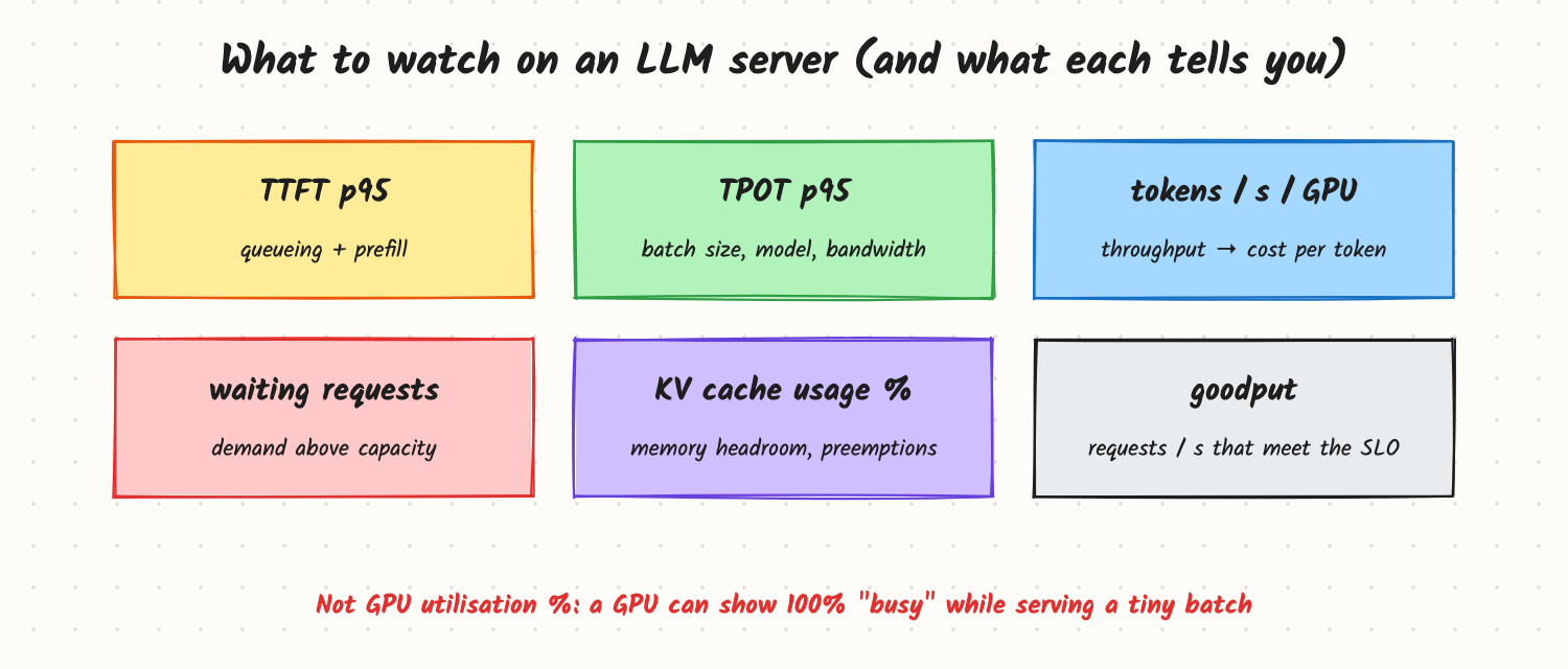
- TTFT (time to first token), p50 and p95: queueing plus prefill. Rises with load and prompt length.
- TPOT (time per output token): decode speed per user. Rises with batch size and model size.
- Throughput: output tokens per second per GPU. Divide GPU cost by it to get cost per token.
- Waiting requests (queue depth): demand the fleet isn't serving yet. The earliest sign you need capacity.
- KV cache usage and preemptions: memory headroom. Near 100% means new requests wait or running ones get evicted.
- Goodput: requests per second that meet the latency SLO (for example TTFT under 1 s and TPOT under 50 ms). Raw throughput can rise while goodput falls.
"GPU utilisation" from standard tools only says a kernel was running, not how much of the GPU it used; a server with a batch of two can show 100%. Use engine metrics (vLLM, SGLang and TensorRT-LLM all export these) instead.
Autoscaling and cold starts
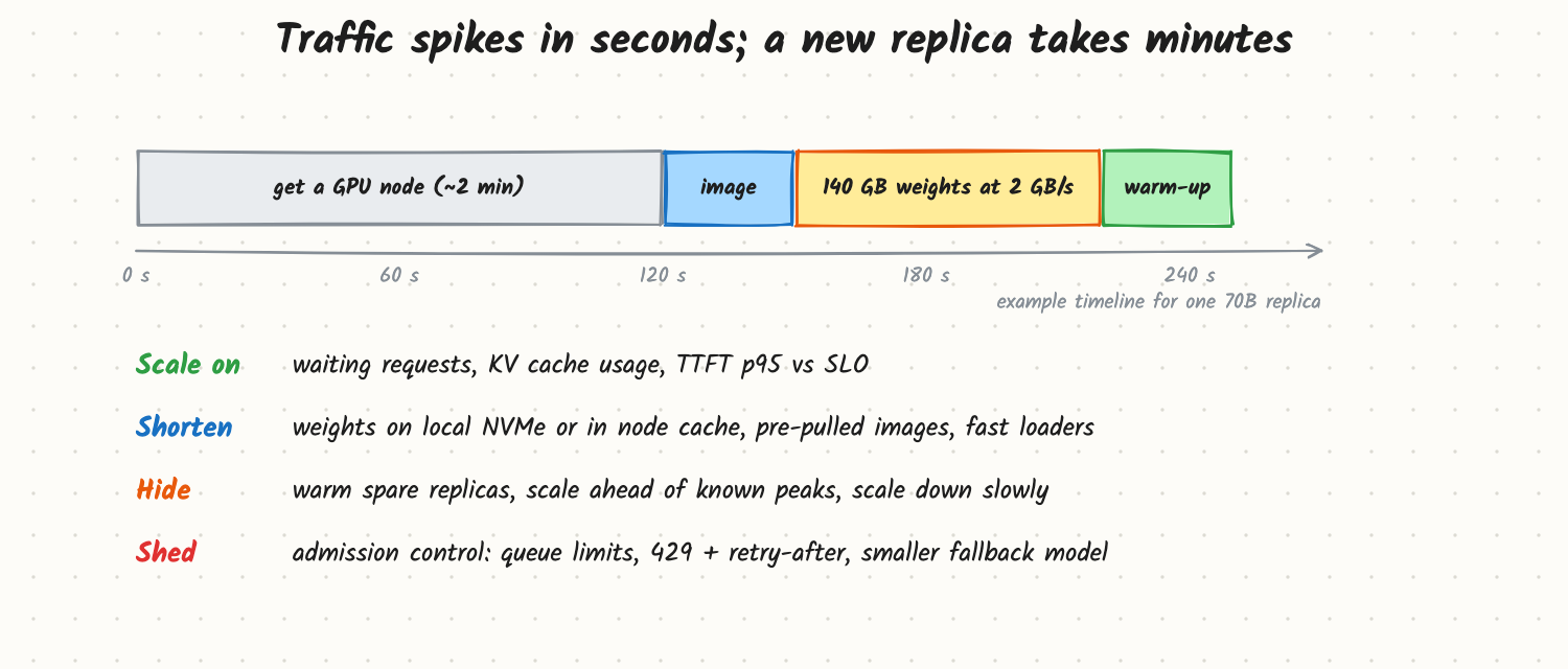
Web servers scale on CPU and start in seconds. LLM replicas start in minutes: get a GPU node, pull a large container image, load the weights (140 GB at 2 GB/s is 70 s; from slow network storage it can be several minutes), then warm up kernels and graphs. So:
- Scale on the right signal: waiting requests per replica, KV cache usage, or TTFT p95 against the SLO. Not CPU, and not GPU utilisation.
- Shorten the cold start: keep weights on local NVMe or a node-level cache, pre-pull images on GPU nodes, use fast parallel loaders or pre-sharded checkpoints.
- Hide it: keep a buffer of warm replicas, scale ahead of known peaks (schedules, launches), and scale down slowly, since a replica you remove is minutes away from coming back.
- Shed load gracefully: cap the queue, return 429 with retry-after, route overflow to a smaller model or a hosted API, and prioritise paying or interactive traffic over batch.
GPU node supply is its own limit: in a busy cloud region the node may not be available at all, so reserved capacity covers the base load and on-demand covers the peaks.
Disaggregated prefill and decode
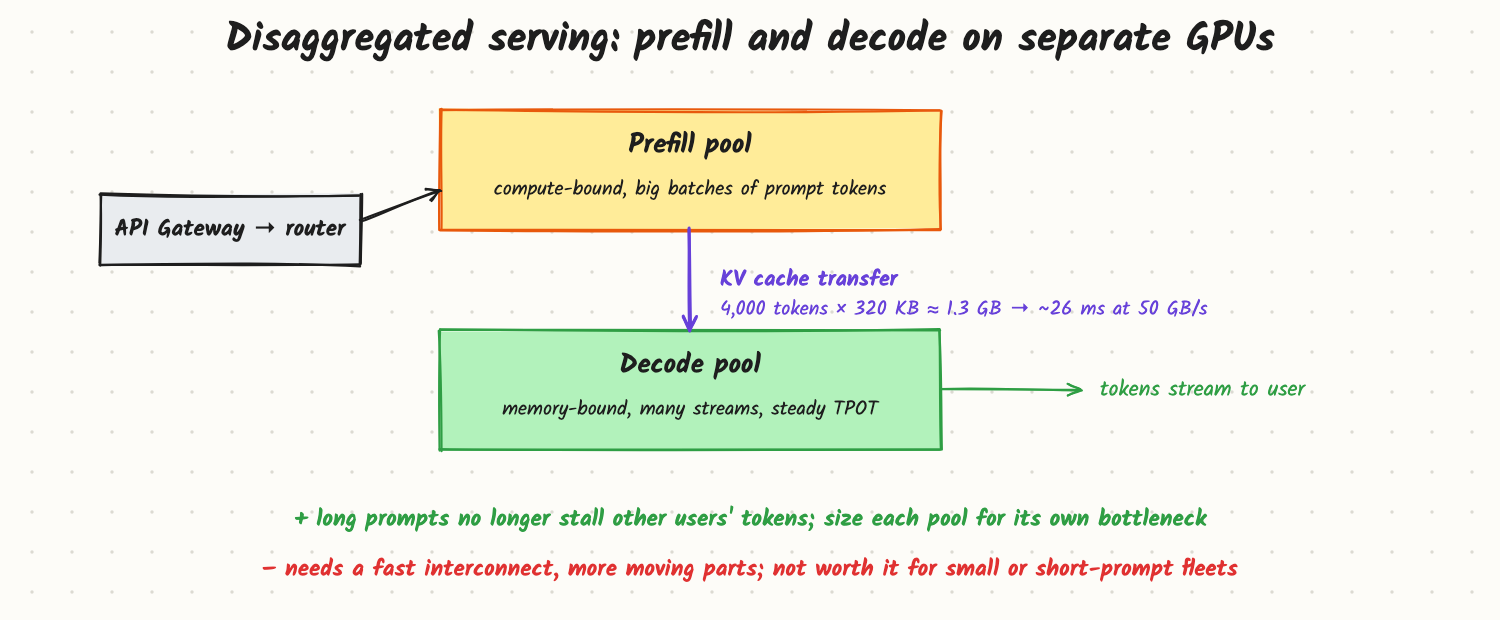
Prefill is compute-bound and bursty; decode is memory-bound and steady. On one GPU they interfere: a 30,000-token prompt's prefill delays every running user's next token. Chunked prefill softens this. Disaggregated serving goes further:
- A prefill pool runs prompts in large batches and produces the KV cache.
- The cache is transferred over a fast network (NVLink, InfiniBand or RDMA) to a decode pool. For a 4,000-token prompt on a 70B model that's about 1.3 GB, roughly 26 ms at 50 GB/s.
- The decode pool streams tokens with stable TPOT, and each pool is sized and scaled for its own bottleneck. The prefill:decode GPU ratio follows your prompt-to-output length mix.
This design (described in research systems such as DistServe and Splitwise, and supported by newer serving stacks) pays off at large scale with long prompts; for a small fleet the transfer and extra moving parts cost more than they save.
Trade-offs and costs
- Headroom vs cost. Warm spare replicas waste money when idle; too few means timeouts at every spike.
- Scaling signals lag differently. Queue depth reacts fastest, latency percentiles are noisy, KV usage depends on context length. Many teams combine queue depth with a latency guard.
- Bigger replicas vs more replicas. Tensor-parallel replicas across several GPUs lower latency per request but scale in larger, slower steps.
- Disaggregation adds network cost and failure modes (a decode node waiting on a slow transfer).
In production
- The usual stack: API Gateway → model router → replicas on Kubernetes with GPU nodes, autoscaled by a custom metric (queue depth or KV usage) rather than CPU.
- Route with awareness of load and cache: least outstanding tokens, plus prefix or session affinity for prefix caching.
- Separate interactive and batch traffic into different priority classes or pools.
- Alert on goodput and TTFT p95, not on GPU utilisation.
When to reach for it
Any self-hosted LLM serving beyond a single box, and every inference-platform design question. Disaggregation is the follow-up for long-prompt, high-volume workloads (RAG, coding assistants, agents) where prefill interference shows up as TPOT spikes.
Example
A RAG assistant runs 12 replicas of a 70B model. Daily peaks are predictable (9–11 am), plus occasional launch spikes. Changes: scale on waiting requests per replica > 4, keep 2 warm spares, schedule +4 replicas at 8:45 am, cache weights on node NVMe (load time from 6 min to 70 s), and send overflow to a smaller fallback model with a banner. Prompts average 12,000 tokens and outputs 400, so the team moves to 4 prefill + 8 decode GPUs per group. TPOT p95 falls from 95 ms to 40 ms during peaks. (Example numbers.)
Common mistakes
- Autoscaling on GPU or CPU utilisation.
- Ignoring cold-start time, so scaling always arrives after the spike.
- Reporting average latency; use p95 and goodput.
- No load shedding, so overload turns into timeouts for everyone instead of quick 429s for some.
- Disaggregating a small fleet where chunked prefill was enough.
Say this in the interview
"I'd measure TTFT and TPOT at p95, tokens per second per GPU, queue depth, KV cache usage and goodput against the SLO, not GPU utilisation. Replicas take minutes to start because of node provisioning and loading 100+ GB of weights, so I'd autoscale on queue depth or KV usage, keep warm spares, pre-scale for known peaks, cache weights on local NVMe, and shed load with 429s or a fallback model. At large scale with long prompts, I'd split prefill and decode into separate pools and transfer the KV cache, so long prompts stop hurting TPOT and each pool scales on its own bottleneck."
Interview questions on this
- Why is GPU utilisation a poor scaling signal for LLM serving? It shows whether a kernel ran, not how full the batch or cache is.
- What is goodput and why prefer it to throughput? Requests meeting the SLO per second; throughput can rise while users get slower answers.
- How do you cut cold-start time for a 70B replica? Local or cached weights, pre-pulled images, fast sharded loading, warm pools.
- What happens at a traffic spike before new replicas arrive? Queues grow; use admission control, priorities and fallbacks.
- Why separate prefill from decode? Different bottlenecks and interference; separate pools give stable TPOT and independent scaling.
- How do you size the prefill-to-decode ratio? From prompt and output length distributions and each pool's measured tokens per second.
Used in
- AI Engineering: Prefill, Decode and the KV Cache; Continuous Batching; Prefix Caching; GPU Utilization and Cost; GPU Job Scheduling and Queues; Model Routing and Fallbacks; How Many GPUs Do You Need to Serve a 70B Model?
- AI System Design: Design an Inference Platform; Design an LLM Gateway; Design ChatGPT.